Usage
[1]:
%matplotlib inline

import glob
import shutil
import tempfile

import matplotlib.pyplot as plt
from astropy.io import fits
from ndcombine import combine_arrays
from ndcombine.tests.helpers import make_fake_data
First, let’s create some fake images with a few sources and cosmic rays. The FITS files are created in a temporary directory:
[2]:
tmpdir = tempfile.mkdtemp()
make_fake_data(10, tmpdir, nsources=15, ncosmics=10, shape=(100, 100))
..........
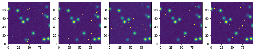
Now we can read the images and plot a few of them:
[3]:
data = [fits.getdata(f) for f in glob.glob(f'{tmpdir}/*.fits')]
len(data)
[3]:
10
[4]:
fig, axes = plt.subplots(1, 5, figsize=(5 * 3, 3))
for ax, arr in zip(axes, data):
    ax.imshow(arr, origin='lower', vmax=1000)
And we can combine the images with the combine_arrays function:
[5]:
out = combine_arrays(data, method='mean', clipping_method='sigclip')
The output of combine_arrays is a NDData object:
[6]:
out
[6]:
NDData([[205.48490906, 195.53549347, 208.11802673, ..., 195.76672058,
         198.55113983, 191.07581482],
        [191.82683716, 208.75389862, 198.61694031, ..., 209.15925598,
         190.55748444, 191.59490051],
        [200.75752411, 197.99489594, 200.71036682, ..., 201.98721466,
         186.91941681, 192.65893707],
        ...,
        [204.41634827, 207.21008759, 201.93208923, ..., 203.25865326,
         200.95804596, 207.46765747],
        [196.69404297, 201.06773071, 202.44575806, ..., 189.55034637,
         204.5367157 , 200.54300385],
        [198.3311615 , 194.67256927, 194.18457031, ..., 196.0560318 ,
         204.5740097 , 204.50482635]])
In its meta dict it also contains an array with the number of values that have been rejected for each pixel:
[7]:
out.meta['REJMAP']
[7]:
array([[0, 0, 0, ..., 0, 0, 0],
       [0, 0, 0, ..., 0, 0, 0],
       [0, 0, 0, ..., 0, 0, 0],
       ...,
       [0, 0, 0, ..., 0, 0, 0],
       [0, 0, 0, ..., 0, 0, 0],
       [0, 0, 0, ..., 0, 0, 0]], dtype=uint16)
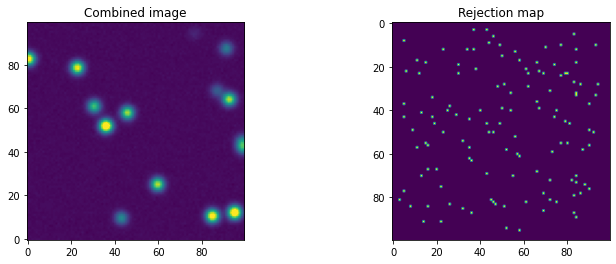
[8]:
fig, (ax1, ax2) = plt.subplots(1, 2, figsize=(2 * 6, 4))
ax1.imshow(out.data, origin='lower', vmax=1000)
ax2.imshow(out.meta['REJMAP'])
ax1.set(title='Combined image')
ax2.set(title='Rejection map');
[9]:
# Cleanup
shutil.rmtree(tmpdir)